Particle Analysis Tutorial

This is a tutorial to show how basic particle analysis by thresholding works. We will select particles by contrast difference with the background, filter by size and measure properties including minimum/maximum/mean diameter, area, circularity and more.

#Import dependancies - here we are looking at particles in a single image, so we use Micrograph() to hold the image

from SimpliPyTEM.Micrograph_class import Micrograph

#This praticle analysis module contains the functions suitable for performing this type of particle analysis
from SimpliPyTEM.Particle_analysis import Threshold, Find_contours, Collect_particle_data

#Import matplotlib to plot the data
import matplotlib.pyplot as plt

#numpy is used for arrays and mathematicl operations
import numpy as np

<Figure size 640x480 with 0 Axes>

Locate files

Here I get a list of files from the directory Particle_analysis_files, these are the fiels I will use for this tutorial. As they are in a different folder from my working directory I need to include a prefix to them, Here I will use pythons generator expression syntax to do this effectively.

import os
files = ['Particle_analysis_files/'+x for x in os.listdir('Particle_analysis_files')]
print(files)

['Particle_analysis_files/CC_15_2021_H_0018.dm3', 'Particle_analysis_files/CC_15_2021_H_0022.dm3', 'Particle_analysis_files/CC_15_2021_H_0016.dm3']

print(os.listdir('.'))

['Example_image_0021_250nmscale.jpg', 'Fibrils_Example.jpg.jpg', 'Output_video.avi', '.DS_Store', 'Fibrils_Example_100nmscale.jpg', 'Cy5.5_A5_0006_0.5umscale.jpg', 'images', '1mfr.cif', 'First_frame.jpg', 'Example', 'Cy5.5_A5_0006.jpg', '1hmr.cif', 'Cy5.5_A5_0006_0.5µmscale.jpg', 'Example-0003_250nmscale.jpg', 'Cy5.5_A5_0006.dm3', 'Frames', 'Fibres_1.jpg', 'Example_image_0021.dm3', 'Fibrils_Example.dm3', 'Output_video.mp4', 'A1_Tribloc-100000X-0003.dm4', 'Fibrils_Example.jpg', '.virtual_documents', 'Particle_plots_new.png', 'Example_image_0021.jpg', 'Particle_data.csv', 'Uneven_contrast.jpg', 'metadata.csv', 'gold_growth_video_holder_test_070921.tif', 'MicrographAnalysisTutorial.ipynb', '.ipynb_checkpoints', 'Particle_analysis_files', 'Old_fibril_oligomers_sample_unstained_0041.dm3', 'Last_frame.jpg', 'imagesTutorial_image.tif_25nmscale.tif', 'MicroVideoAnalysisTutorial.ipynb', 'gold_growth_video_holder_test_070921_25nmscale.jpg', 'Fibres_1_25nmscale.jpg', 'Particle_analysis_tutorial.ipynb', 'A1_Tribloc-100000X-0003_250nmscale.jpg', 'Video_averaged.jpg', '__temp__.mp4', 'gold_growth_video_holder_test_070921.dm4']

Open Micrograph

For now we are only going to focus on one of the 3 files, we will come back to the others later though.

im = Micrograph(files[0])

Particle_analysis_files/CC_15_2021_H_0018.dm3 opened as a Micrograph object

#Lets see how it looks
im.imshow()

So we can see particles, but the contrast is pretty poor, while we dont have to, its best to improve this before continuing with the analysis. Lets move do this with a preprocessing step.

Preprocess image

First thing to do is check how this histogram looks:

im.plot_histogram(sidebyside=True)

Now although it is not strictly neccessary, I prefer working with 8-bit images, this is standard for images and has the pixel values scaled between 0-255. It also improves the contrast enhancement.

im8bit = im.convert_to_8bit()
im8bit.plot_histogram(sidebyside=True)

Next I want to normalise contrast across the image. This is particularly important if there is uneven contrast in the image. We are going to detect particles by thresholding, which makes it important that the contrast in the image is uniform. If for example, the corners of the image are darker than the center, possibly due to a missaligned beam or aperture, it can become difficult to separate the particles effectively. Here I use local normalisation (see micrograph tutorial) to perform this. You may notice there is a patchwork effect produced by this, while this can be avoided by running with padding (pad=True), in my experience, this effect does not cause an issue.

im8bitLN= im8bit.local_normalisation(6)
im8bitLN.plot_histogram(sidebyside=True)

Next I gaussian filter - this smooths the edges of the particles to make them easier to threshold.

im8bit_gaussian= im8bitLN.gaussian_filter(5)
im8bit_gaussian.plot_histogram(True)

Finally, I am going to improved the contrast using the clip_contrast method:

im8bit_clipped = im8bit_gaussian.clip_contrast(saturation=0.1)
im8bit_clipped.plot_histogram(True)
im_processed = im8bit_clipped

Saturation =  0.1
Maxmium value :  172.0
Minimum value :  78.0

The local normalisation patchwork effect has finally been seen, this shouldnt cause an issue though.

If you have a large image, particle picking can become slow. You may want to bin image (reduce the size) to speed up particle picking, I’m going to skip this here but I’ve left the code here:

#im_processed = im8bit_clipped.bin(2)
#im_processed.plot_histogram(True)

Thresholding

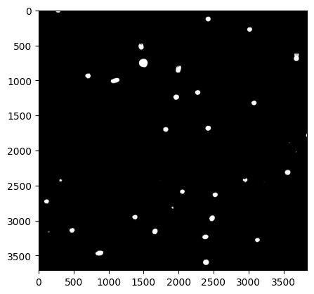
The first step when analysing particles is to separate the particles from the background. The most common method for this is by simply thresholding, this chooses a value. Anything under this value is set to black (0), whilst anything above the value is set to white.

SimpliPyTEM’s thresholding implementation automataically erodes and dilates the threshold to improve the resultss. Using this function is optional however, you can explore using tricks using other image analysis methods to best threshold your image. The key point here is that the output is a binary image with the particles as white and the background as black.

This implementation also assumes your image is brightfield, i.e. the particles are dark and the background is light. This assumption can be reversed by setting brightfield=False as a parameter,

Finding a good threshold value is guided by the histogram and by trial and error:

thresh = Threshold(im_processed.image, 100)

plt.imshow(thresh)
plt.show()

How do thresholds compare? Here I will crop a small region of the image showing a particle and compare how different threshold values make the particle appear.

thresholds = [100, 110,120,135,150]
fig, ax = plt.subplots(1,6, figsize =(40,10))
ax[0].imshow(im_processed.image[400:900, 1300:1700])
for i in range(len(thresholds)):
    ax[i+1].imshow(Threshold(im_processed.image, thresholds[i])[400:900, 1300:1700])
    ax[i+1].set_title('Threshold = {} '.format(thresholds[i]))

plt.show()

Here we see that increasing the threshold value leads to more noise being selected which may cause issues with falsely selecting particles. This image has very high contrast particles which makes this step easier. Here I will choose a threshold of 120, as some surrounding noise is ok, because we will filter by size, its best to pick up the full particle. Lets solidify this then:

threshold = 120
thresh= Threshold(im_processed.image, threshold)
plt.imshow(thresh)
plt.show()

Locating particles

Using a function called ‘Find_contours’ which locates the edges of the particles. This also filters the particles by size - a minimum area (in number of pixels) is given. It will also remove particles on the edge of the image. A max size can also be added (using the maxsize parameter) if required, here we are only interested in the minimum size but there may be images with aggregates and similar large items which you may not want to select. This returns two objects:

- contours_im is a list of arrays containing the coordinates which define the particles selected.
- mask is a binary image showing particles in white.

Find_contours has been updated in SimpliPyTEM version 1.0.9 with a massive speed boost, so if it is running slowly, double check your version number.

contours_im, mask =Find_contours(thresh, minsize=300)

The speed boast mentioned above consisted of A) making the code more efficient and B) Running multiple processes simultaneously for the slowest step.

You can adjust this second parameter as follows:

import time
start = time.time()
contours_im, mask = Find_contours(thresh, minsize=200, threads=1)
print('Running time for 1 thread: ', time.time()-start)
start = time.time()
contours_im, mask = Find_contours(thresh, minsize=200, threads=2)
print('Running time for 2 threads: ', time.time()-start)
start = time.time()
contours_im, mask = Find_contours(thresh, minsize=200, threads=5)
print('Running time for 5 threads: ', time.time()-start)
start = time.time()
contours_im, mask = Find_contours(thresh, minsize=200, threads=10)
print('Running time for 10 threads: ', time.time()-start)

Running time for 1 thread:  6.716806173324585
Running time for 2 threads:  4.438666820526123
Running time for 5 threads:  3.142490863800049
Running time for 10 threads:  2.807776927947998

More threads are not always better, in my experience 5 is about optimal on the two computers tested and so this has been set as the default value, and thus this can in most cases be ignored. This value can be optimised to improve this though.

For context, these runnning time values were using my (admittedly quite powerful) MacbookPro 2018. If this step is still running too slowly for you, try binning the image with Micrograph.bin(), I get a >10x speed increase with a 2X xy bin.

As I mentioned above, its ok when thresholding to pick up small noise specs because they are filtered out in this step (see below), however for maximum speed you can also have a harsher threshold as Find_contours total running time depends heavily on the number of individual particles (or specs of noise) which are in the thresholded image.

#Lets compare the mask to the original using the micrograph.show_pair() function

im_processed.show_pair(mask)

Now theres a few very small particles that I’m not convinced are real (e.g. see bottom left, around 50,3200), now this could be a different populataion that I am interested in, but here I’m not interested in these We can filter this out by raising the minimum size parameter:

contours_im, mask =Find_contours(thresh, minsize=750)
im_processed.show_pair(mask)

This looks like it gets everything that I think is a particle, without selecting anything else which is the ideal scenario. Lets move on with this.

Collecting and plotting paraticle data

Uses Collect_particle_data() function with two inputs: the contours_im defined in the last section and the pixel size of the image, which can be located from the micrograph object im_processed (remember that the image has been binned so its important to use im_processed rather than im)

The data collected will be in the same unit as the pixel_size input that you give.Having the pixel_size attribute saved in the micrograph object is quite useful here. You may want to double check that the pixel_unit is what you expect though. Here I want to work in nanometers, lets first see if thats what I have.

print(im_processed.pixel_size, im_processed.pixel_unit)

# Good thing I checked! I want it in nanometers, so lets change that:

im_processed.change_scale_unit('nm')
print(im_processed.pixel_size, im_processed.pixel_unit)

0.0013585201231762767 µm
1.3585201231762767 nm

Now we can use this to collect correctly scaled data:

data = Collect_particle_data(contours_im, im_processed.pixel_size)

The data is in a dictionary with keys being the features described. To see the features available use data.keys()

print(data.keys())

dict_keys(['Area', 'Centroid', 'Centroid_x', 'Centroid_y', 'Perimeter', 'Circularity', 'Width', 'Height', 'Radius', 'Major-Minor Ratio'])

Some of these features are pretty self explanatory but lets go through them here:

Area - The area of the particle in the image
     Centroid - The center point coordinate of the particle (x, y)

Circularity - The area of the particle divided by the area of a circle that completely bounds the particle, giving a value for how circular it is (or how much of a circle it fills)

Width - The width of the smallest possible rectangle that could fully contain the particle

Height - The height of the smallest possible rectangle that could fully contain the particle

radius - The radius of the smallest possible circle that could fully contain the particle.

Major-Minor Ratio  - The ratio between height and width

To use the individual data, use these keys:

print(data['Width'])

[89.19839441966192, 61.416071259479565, 93.96410813576317, 97.283885966978, 103.24752936139703, 96.08593555928823, 98.08515911213877, 100.53048911504447, 165.37043074722035, 103.65338973572058, 98.53520414287331, 49.142728334528485, 106.63036594222586, 98.84685988615783, 89.66232812963426, 96.7619411094729, 97.73374443336458, 113.45709746909982, 98.04540017664908, 97.8992684687583, 104.9694871991056, 97.11602987723467, 87.01491784381865, 91.47343263161467, 91.05423290641124, 86.98523338311936, 105.8202309905365, 100.53048911504447]

We can plot some of this data using matplotlib:

plt.hist(data['Width'], bins=20)
plt.xlabel('Particle Width')
plt.ylabel('Frequency')
plt.show()

Now before we move on from here, There is an additional parameter for Collect_particle_data called multimeasure. This uses an additional function to measure the particles diameter at many different positions around the particle, the maximum, minimum, mean and standard deviation of the diameter are then kept, along with the number of measurements per particle:

data = Collect_particle_data(contours_im, im_processed.pixel_size, multimeasure=True)
print(data.keys())

WARNING:py.warnings:/Users/gabriel/python_imageanalysis/Micrograph_analysis_scripts/SimpliPyTEM/Particle_analysis.py:516: RuntimeWarning: invalid value encountered in arccos
  angle = np.degrees(np.arccos(cosine_angle))

dict_keys(['Area', 'Centroid', 'Centroid_x', 'Centroid_y', 'Perimeter', 'Circularity', 'Width', 'Height', 'Radius', 'Major-Minor Ratio', 'Min diameter', 'Max diameter', 'Mean diameter', 'Stddev diameter', 'Measurements'])

print(data['Measurements'])

[88, 60, 92, 104, 222, 222, 108, 98, 202, 66, 60, 34, 120, 162, 62, 126, 140, 120, 96, 84, 78, 104, 166, 98, 88, 98, 122, 162]

Here we have plenty of measurements, however sometimes there are very few measurements, particularly with small particles.

To improve this, we can go back a step and redo the Find_contours() step with complex_coords=True. The resulting contours will be better defined as it will no longer try to remove the redundant coordinates of the edges, see OpenCV’s contours documentation for more details.

The multimeasure should then have more coordinates to work with and thus have more measurements, the downside here is that evrything will take longer to run however.

contours_im, mask =Find_contours(thresh, minsize=750, complex_coords=True)
data = Collect_particle_data(contours_im, im_processed.pixel_size, multimeasure=True)
print(data['Measurements'])

[296, 194, 300, 336, 744, 762, 340, 448, 830, 402, 308, 140, 476, 548, 264, 398, 584, 496, 320, 404, 358, 406, 402, 312, 352, 306, 518, 628]

See? loads more measurements…

Plotting data

Now we just need to plot the data! Here is an example plot I have made with the seaborn and matplotlib libraries. I’m not going to go into the details of this too much, if you dont know much about plotting data in python I recommend you look at the matplotlib and/or seaborn libraries for inspiration. Or you can skip this step and export the data to a .csv file below.

import seaborn
import matplotlib
import matplotlib.pyplot as plt

#Get data
hdata= data['Max diameter']
wdata = data['Min diameter']
mdata = data['Mean diameter']
cdata= data['Circularity']
xpos = data['Centroid_x']
ypos = data['Centroid_y']



#Change global parameters
matplotlib.rcParams['font.size']=30
matplotlib.rcParams['axes.linewidth'] = 4
matplotlib.rcParams['lines.linewidth'] = 4

#Create a figure with 3 subplots
fig, ax = plt.subplots(1,3,figsize=(30,10))

#plt.tight_layout()

#Make Ticks bigger
for a in ax:
    a.xaxis.set_tick_params(width=5, length=10)
    a.yaxis.set_tick_params(width=5, length=10)

#Set the seaborn color palette to be my color palette
colors = ['#F2B8D5', '#95A9C1','#C2E4E9','#D8BBEA','#E5E8B5']
seaborn.set_palette(seaborn.color_palette(colors))

#Plot the diameter violin plot
seaborn.boxplot([wdata, hdata,mdata] ,ax=ax[0], linewidth=4)

#Set violin plot labels and limits
ax[0].set_ylim(50,200)
ax[0].set_title('Diameter', fontsize=40)
ax[0].set_ylabel('Particle Diameter (nm)')
ax[0].set_xticklabels(['Minimum', 'Maximum', 'Mean'])

#Plot histogram of Circularity
ax[1].hist(cdata, color='#D8BBEA',edgecolor='black',linewidth=4, bins=6)
ax[1].set_title('Circularity', fontsize=40)
ax[1].set_xlabel('Circularity')
ax[1].set_ylabel('Frequency')
ax[1].set_xticks([x/10 for x in range(4,11)])
ax[1].set_xlim(0.35,1)

#Add a line to show the mean
ax[1].axvline(np.mean(cdata), color='red')
label='Mean = ' +str(round(np.mean(cdata),2))
ax[1].annotate(label, (0.6,10), fontsize=20)

#Plot the positions of the particles on a scatter plot
ax[2].scatter( xpos, ypos , color='#E5E8B5', marker='o',edgecolors='black',s=150, linewidth=3)
ax[2].set_title('Position', fontsize=40)
ax[2].set_ylabel('')
ax[2].set_xlabel('')
ax[2].set_xlim(0, 1919)
ax[2].set_ylim(1855,0)

#Show plot (can also use plt.savefig('Name.png') to save the figure)
plt.savefig('Particle_plots_new.png')
#plt.show()

Using multiple files

What if we want to use multiple images, maybe with different pixel sizes, how can we deal with that?

Firstly lets remember the files that we have:

print(files)

['Particle_analysis_files/CC_15_2021_H_0018.dm3', 'Particle_analysis_files/CC_15_2021_H_0022.dm3', 'Particle_analysis_files/CC_15_2021_H_0016.dm3']

We want to preprocess the files again, lets not go through it one by one though, lets just make a preprocess function that we can use for each file. We are also going to create a function to plot a range of thresholds like we did before:

def preprocess(im, binn=True):
    im = im.convert_to_8bit()
    im = im.local_normalisation(6)
    im = im.gaussian_filter(9)
    im = im.clip_contrast(saturation=0.05)
    im = im.bin()
    return im

def plot_thresholds(im):
    thresholds = [100, 110,120,135,150]
    fig, ax = plt.subplots(1,6, figsize =(30,5))
    ax[0].imshow(im_processed.image)
    for i in range(len(thresholds)):
        ax[i+1].imshow(Threshold(im.image, thresholds[i]))
        ax[i+1].set_title('Threshold = {} '.format(thresholds[i]),fontsize=20)
        ax[i+1].set_xticks([])
        ax[i+1].set_yticks([])
    plt.show()

Thresholds need to be manually decided but that doesn’t stop us looping over the files for preprocessing. I will use the functions created above to preprocess and then plot the thresholds and decide the thresholds from here.

processed_ims = []
for file in files:
    print(file)
    im = Micrograph(file)
    im_processed = preprocess(im)
    processed_ims.append(im_processed)
    plot_thresholds(im_processed)

Particle_analysis_files/CC_15_2021_H_0018.dm3
Particle_analysis_files/CC_15_2021_H_0018.dm3 opened as a Micrograph object
Saturation =  0.05
Maxmium value :  190.0
Minimum value :  59.0

Particle_analysis_files/CC_15_2021_H_0022.dm3
Particle_analysis_files/CC_15_2021_H_0022.dm3 opened as a Micrograph object
Saturation =  0.05
Maxmium value :  182.0
Minimum value :  41.0

Particle_analysis_files/CC_15_2021_H_0016.dm3
Particle_analysis_files/CC_15_2021_H_0016.dm3 opened as a Micrograph object
Saturation =  0.05
Maxmium value :  207.0
Minimum value :  47.0

Now if this is in a jupyter notebook, one can doubleclick on each figure and get a closer look. Here though I have decided for each image what I think the suitable thresholds should be. Now I will save these in a list, these should be the same order as the files in the files list.

One thing to note here is that the particles are filled in in the find_contours function. Therefore the key is getting the edges right. In some of these images, the full particle is not selected but as long as the outline is, we can proceed to the next step.

thresholds = [120, 130, 120]

Now, remember how the the pixel size of the image was in µm and I wanted it in nanometers? Lets make sure this is fixed for all images. I’m going to do this with the change_scale_unit() method, this will skip the file if the unit is already correct so I can run it on each file without worrying.

for im in processed_ims:
    print(im.filename)
    print('Starting pixel_size = {}{}'.format(str(round(im.pixel_size,3)),im.pixel_unit))
    im.change_scale_unit('nm')
    print('New pixel_size = {}{}'.format(str(round(im.pixel_size,3)),im.pixel_unit))
    print('\n')

Particle_analysis_files/CC_15_2021_H_0018.dm3
Starting pixel_size = 0.003µm
New pixel_size = 2.717nm


Particle_analysis_files/CC_15_2021_H_0022.dm3
Starting pixel_size = 1.257nm
The unit is already nm! Skipping file.
New pixel_size = 1.257nm


Particle_analysis_files/CC_15_2021_H_0016.dm3
Starting pixel_size = 0.902nm
The unit is already nm! Skipping file.
New pixel_size = 0.902nm

So now we have a list of pre-processed images and a list of threshold values to use. We can finally get down to it!

Before we start, we need to create empty lists to store the data. We will then append the data and the masks.

Now in these images we have different magnifications so the areas in pixels are completely different, making it difficult to use a single minsize value, so I am also going to define different minimum sizes for each image.

minsizes = [700, 2000,2000]

#create lists to store data
masks = []
alldata = []

for i in range(len(processed_ims)):
    #define which image we are working on (just to make code look neater!)
    im = processed_ims[i]

    #Threshold
    thresh = Threshold(im.image, thresholds[i])

    #Find contours
    contours_im, mask = Find_contours(thresh, minsize=minsizes[i])

    #Plot mask to check
    im.show_pair(mask)


    #Collect data
    data = Collect_particle_data(contours_im, im.pixel_size, multimeasure=True)

    #Save the data to the empty lists we created
    alldata.append(data)
    masks.append(mask)

WARNING:py.warnings:/Users/gabriel/python_imageanalysis/Micrograph_analysis_scripts/SimpliPyTEM/Particle_analysis.py:516: RuntimeWarning: invalid value encountered in arccos
  angle = np.degrees(np.arccos(cosine_angle))

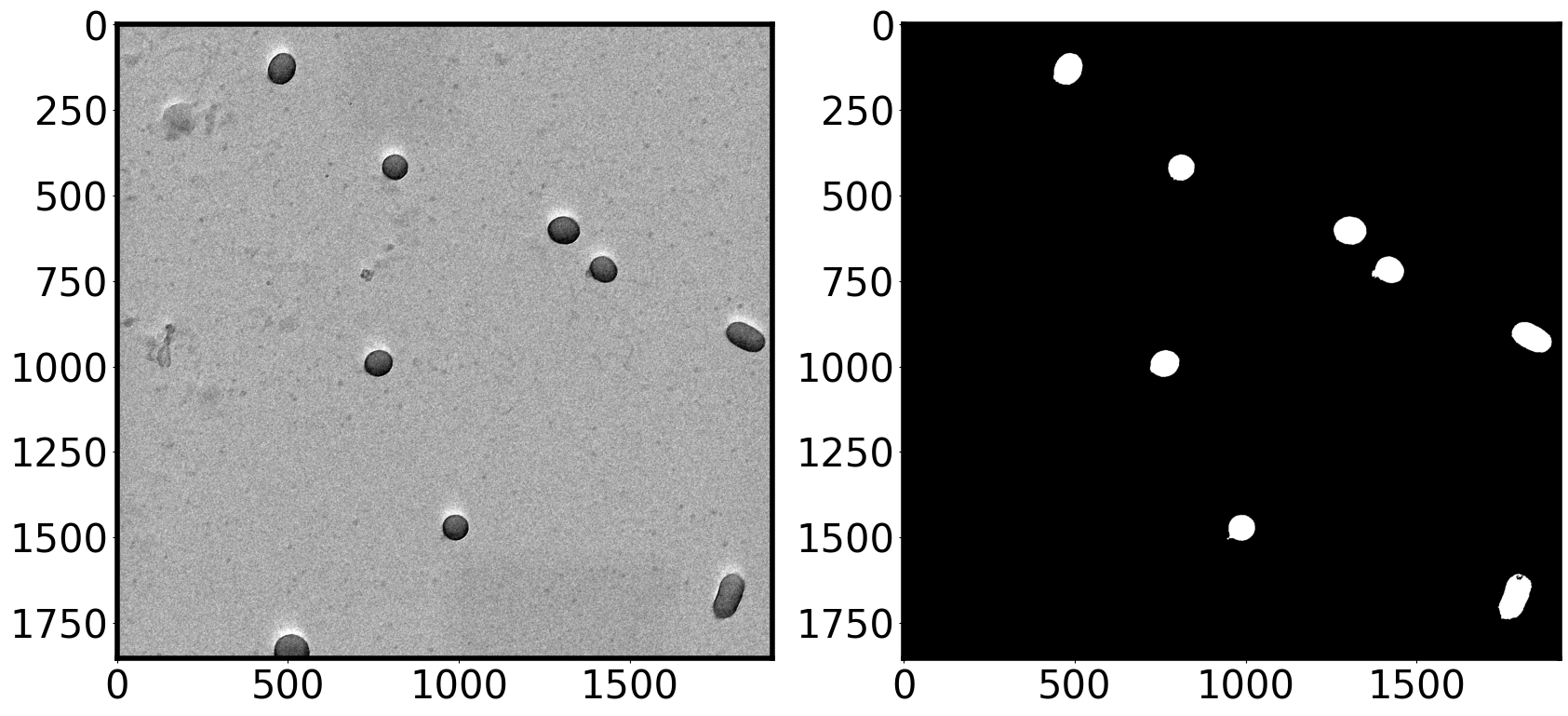
So, now we have the masks shown above saved if we want them again, and more importantly we have the data in the list alldata. Now this is a list of dictionaries, we will make this into one dataset in a second, but first, lets see if the particles have similar sizes across the images:

means = [x['Mean diameter'] for x in alldata]

fig,ax = plt.subplots(figsize=(10,10))

seaborn.boxplot(data=means)
ax.set_ylabel('Particle Diameter (nm)')
ax.set_xticklabels(['Image1','Image2','Image3'])
plt.show()

Looks good! there are only a few particles in the second and third image, so not going to get great statistics or identical means, but they are definitely scaling correctly! Now lets join the data together:

Joining data together

Now we have a list of dictionarys - we can make this into one dictionary like this:

# make an new empty dictionary
alldata_dict = {}

#Create empty options for each key value
for key in alldata[0].keys():
    alldata_dict[key]= []

#Append the data from each dataset into the new dictionary
for dset in alldata:
    for key in dset:
        alldata_dict[key].append(dset[key])

This puts it into one dictionary, the only problem is the data in each category is split into lists from each image. This can be fixed using one confusing line of code, or alternatively the function Flatten_list(). You can see this if you look below.

#Check the condition at the start
print('There are {} datasets in the dictionary'.format(len(alldata_dict['Width'])))

There are 3 datasets in the dictionary

width_data = [x for i in alldata_dict['Width'] for x in i]
print('There is now a single dataset with {} datapoints'.format(len(width_data)))

#or more conveniently:

#Import the function
from SimpliPyTEM.Particle_analysis import Flatten_list

width_data = Flatten_list(alldata_dict['Width'])
print('There is now a single dataset with {} datapoints'.format(len(width_data)))

There is now a single dataset with 37 datapoints
There is now a single dataset with 37 datapoints

To simplify things, there is a function called Convert_to_single_dict which does this last couple of steps for you. The parameter combine_data defines whether you want too combine the datasets (or flatten the lists) as above, or keep them separate, here I will be keeping them separate.

#import the function
from SimpliPyTEM.Particle_analysis import Convert_to_single_dict
alldata_dict = Convert_to_single_dict(alldata, combine_data=False)

Now lets make a similar plot as we did for the single image, except this time, lets colour the positions by which image they are from:

#Get data
hdata= Flatten_list(alldata_dict['Max diameter'])
wdata = Flatten_list(alldata_dict['Min diameter'])
mdata = Flatten_list(alldata_dict['Mean diameter'])
cdata= Flatten_list(alldata_dict['Circularity'])

#get x and y positions
xpos =alldata_dict['Centroid_x']
ypos =alldata_dict['Centroid_y']

#Create a figure with 3 subplots
fig, ax = plt.subplots(1,3,figsize=(45,15))

#Change global parameters
matplotlib.rcParams.update({'font.size': 40}, )
matplotlib.rcParams['axes.linewidth'] = 4
matplotlib.rcParams['lines.linewidth'] = 4

#Make Ticks bigger
for a in ax:
    a.xaxis.set_tick_params(width=5, length=10)
    a.yaxis.set_tick_params(width=5, length=10)

#Set the seaborn color palette to be my color palette
colors = ['#F2B8D5', '#95A9C1','#C2E4E9','#D8BBEA','#E5E8B5']
seaborn.set_palette(seaborn.color_palette(colors))

#Plot the diameter violin plot
seaborn.boxplot([wdata, hdata,mdata] ,ax=ax[0], linewidth=4)

#Set violin plot labels and limits
ax[0].set_ylim(50,220)
ax[0].set_title('Diameter', fontsize=50)
ax[0].set_ylabel('Particle Diameter (nm)')
ax[0].set_xticklabels(['Minimum', 'Maximum', 'Mean'])

#Plot histogram of Circularity
ax[1].hist(cdata, color='#D8BBEA',edgecolor='black',linewidth=4, bins=6)
ax[1].set_title('Circularity', fontsize=50)
ax[1].set_ylabel('Frequency')
ax[1].set_xticks([x/10 for x in range(4,11)])
ax[1].set_xlim(0.35,1)

#Add a line to show the mean
ax[1].axvline(np.mean(cdata), color='red')
label='Mean = ' +str(round(np.mean(cdata),2))
ax[1].annotate(label, (0.6,10), fontsize=30)

#Plot the positions of the particles on a scatter plot
ax[2].scatter( xpos[0], ypos[0] , color='#E5E8B5', marker='o',edgecolors='black',s=300, linewidth=3)
ax[2].scatter( xpos[1], ypos[1] , color='#D8BBEA', marker='o',edgecolors='black',s=300, linewidth=3)
ax[2].scatter( xpos[2], ypos[2] , color='#95A9C1', marker='o',edgecolors='black',s=300, linewidth=3)
ax[2].set_title('Position', fontsize=50)
ax[2].set_ylabel('')
ax[2].set_xlabel('')
ax[2].set_xlim(0, 1919)
ax[2].set_ylim(1855,0)

#Show plot (can also use plt.savefig('Name.png') to save the figure)
plt.show()

Well we haven’t changed much as there were only a few extra particles in the next images, but the satistics have improved and the data is similar!

Saving data

Here I make it into a Pandas dataframe and save it as a .csv file

Pandas is a python module which is excellent for handling data in ‘dataframes’, theses are analogous to an excel spreadsheet.

Before doing anything, lets go back and ensure that the dictionary (alldata_dict) has all the data in a single list:

alldata_dict = Convert_to_single_dict(alldata, combine_data=True)

Now we have a standard dictionary for our data, we can convert it to a dataframe as follows:

import pandas as pd
df = pd.DataFrame(alldata_dict)

#Lets have a look at the result - this prints the first 5 lines
df.head()

	Area	Centroid	Centroid_x	Centroid_y	Perimeter	Circularity	Width	Height	Radius	Major-Minor Ratio	Min diameter	Max diameter	Mean diameter	Stddev diameter	Measurements	Image number
0	5813.567314	(56.11851851851851, 1365.2266666666667)	56.118519	1365.226667	296.576702	0.806028	83.841717	92.347393	47.914979	1.101449	81.556479	92.419316	86.857312	3.910298	14	0
1	6795.414238	(237.8743436538113, 1571.0298750678978)	237.874344	1571.029875	323.747104	0.836122	87.201752	101.465228	50.862551	1.163569	82.769448	101.517001	94.501405	5.783739	24	0
2	7456.130777	(351.60874587458744, 469.98448844884484)	351.608746	469.984488	327.589579	0.842329	92.379368	103.247529	53.081211	1.117647	92.419316	104.137457	100.042667	3.670795	14	0
3	10970.109243	(433.4008524001794, 1733.7206146253923)	433.400852	1733.720615	420.355135	0.580909	92.379368	152.154254	77.531194	1.647059	97.207787	153.554846	128.412468	17.663556	40	0
4	12199.263475	(545.3263741805345, 503.4704992435704)	545.326374	503.470499	456.802094	0.527587	87.409346	171.037261	85.791647	1.956739	87.621915	169.461432	140.797420	28.887768	38	0

Finally, lets save the data as a .csv (comma-separated values) file, this is easy to open with a text editor, excel, python or many other programs that you may wish to use:

df.to_csv('Particle_data.csv')